Sorting, Filtering and Hiding Data in Excel
Spreadsheets can be daunting without the right tools. Here we will go through a few functions in Excel that will help you quickly find that data point you have been so desperately searching for. Through the sort, filter, and hide functions you can cut out a lot of excess noise.
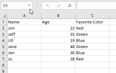
Here we have a small data set. Nothing is in any kind of particular order, but we would really rather it was alphabetized. This is where the sort function comes in. There are a couple of ways to sort a set of data in Excel. Let’s look at one method.
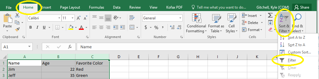
First, select the columns that you would like sorted. A quick way to do this is by clicking on the first column and then holding Shift and clicking on the last column. In the example screenshot below, we clicked on “A”, held down Shift, and clicked “C” in order to select columns A through C for all rows.
Next, in the Home tab click on the Sort & Filter button and then click Filter.
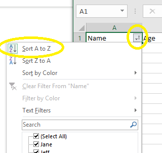
Now you will see a drop down button/arrow button at the top of each of the columns on the spreadsheet. This method works better than clicking on the Sort buttons under Sort and Filter because it sets up the sheet for multiple functions at once which we will cover momentarily.
Now click on the arrow over the column you wish to sort by, and click Sort. In this example, we wanted to sort alphabetically by name so we will click on the arrow by Name, then Sort A to Z.
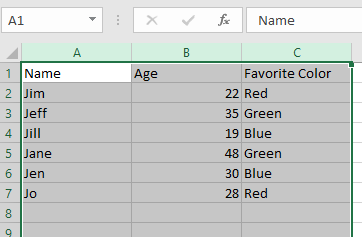
Let’s look at our sample data set again.
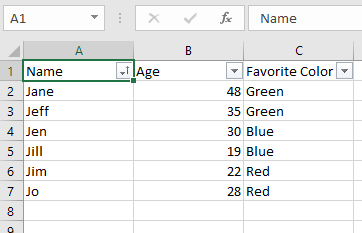
The sort function not only sorted the names alphabetically, but also the data in the rows associated with them! This could be done for the Age or Favorite Color columns as well.
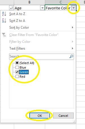
Now that we have the sorting mastered, let’s try filtering this data a bit. We prefer green, so those are the only people we want to see in our data. To do this, we will use the filter function.
Click on the arrow in the Favorite Color column and uncheck the boxes of the data you do not wish to see. Alternatively, you could click the “Select All” box to uncheck everything and then check the ones you want. After making your selection, click “Ok.”
Let’s have another look at that data set.

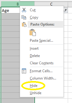
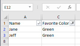
Now we are seeing the data we really care about. Now we want to take a screenshot of this, but Jeff is really sensitive about his age. We can make it disappear from the display without deleting the data in that column using the hide function.
Right click on the column you want to hide and then click “Hide.” You can hide multiple columns this way if you have them all selected.
One last look at the data set.
If you want to see the hidden information again, simply right click on the space the column should be and click “Unhide.”
Now you are ready to trim down those spreadsheets and start getting to the heart of your data.
Remember, if you need assistance or have questions about reporting you can always contact your HMIS Team at Commerce.